
I reproduced a 2018 methylation paper. The authors were right, and their evidence could not show it.
Yassine El Hallaoui · Founder, CEO & CTO · AlkhemYst-Ai · 2026-08-14
I reproduced a 2018 methylation paper. The authors were right, and their evidence could not show it.
Last week I took a published study, rebuilt its analysis from the deposited data, and then ran the tests the authors did not run. I want to describe what happened, because the result is not the one I expected and the interesting part is not the finding.
The paper is Hjorthaug, Gervin, Mowinckel and Munthe-Kaas, Exploring the influence from whole blood DNA extraction methods on Infinium 450K DNA methylation [1], PLoS ONE 2018. It comes from Oslo University Hospital and the University of Oslo. The design is simple and clean. Ten healthy blood donors. DNA extracted from each donor three different ways: magnetic beads on a MagNA Pure, salting out with isopropanol precipitation on an Autopure, and manual organic extraction. Every sample measured on the Infinium 450K array. After quality control, 440,110 probes.
The question is one that matters to anyone running an epigenome wide study on banked blood. Studies pool samples collected over years, from different biobanks, extracted by whatever protocol was in use at the time. If the extraction method itself shifts methylation, every one of those studies has a confounder sitting in it.
Their answer was no. No CpG site and no region reached genome wide significance between methods. Extraction method, they wrote, is "unlikely to confound Infinium 450K methylation analysis in whole blood".
I picked this paper precisely because it looks solid. The data is public on Zenodo. The methods section is detailed enough to reimplement without guessing. And the conclusion is a negative one, which is the hardest kind to support properly and the kind most often reported without the caveat that matters.
---
Getting back to their numbers
The first thing to establish is whether you are analysing the same thing they analysed. This is easy to get wrong and easy to not notice.
Their data ships as an R table, space separated, with the study design encoded in the column headers. The columns are named 1M, 1A, 1O, 2M, 2A, 2O and so on up to 10O. Ten donors, three methods, thirty samples. Nothing in the file says "donor" or "method" anywhere. You have to take the header apart before you can test anything.
Once that is done, 440,110 probes across 30 samples gives 13,203,300 measurements. Each pairwise comparison between two methods, within donor, gives 4,401,100 paired values.
That number appears in their methods section. They write about plotting "each of the 4,401,100 average intra-individual DNA methylation values (10 subjects of 440,110 values each)". Seeing my reproduction return exactly that figure was the moment I trusted it.
The rest matched too. Bias between methods below 0.002 on the beta scale in all three comparisons. Zero CpG sites significant at a 5 percent false discovery rate, in all three comparisons. Their result, rebuilt from their data.
---
A detour that turned into the best part
Their Bland Altman analysis [2] does something unusual. Standard Bland Altman draws limits of agreement as the mean difference plus or minus 1.96 standard deviations, which assumes the differences are normally distributed. They tested that assumption, found it did not hold, and replaced the flat limits with a curve fitted to the data.
I wanted to see how much that decision was worth, so I ran their analysis again with the standard flat limits and nothing else changed.
The bias figures did not move by a single digit, which is correct: a bias does not depend on how you draw the interval around it. What changed is whether the interval describes anything real. The Shapiro Wilk test on the differences returned p values of 2.4e-56, 1.5e-58 and 5.0e-59.
Those are not borderline. The differences are about as far from normal as a distribution gets. Their unusual choice was the right one, and anyone reaching for textbook Bland Altman limits on methylation beta values is drawing an interval the data does not support.
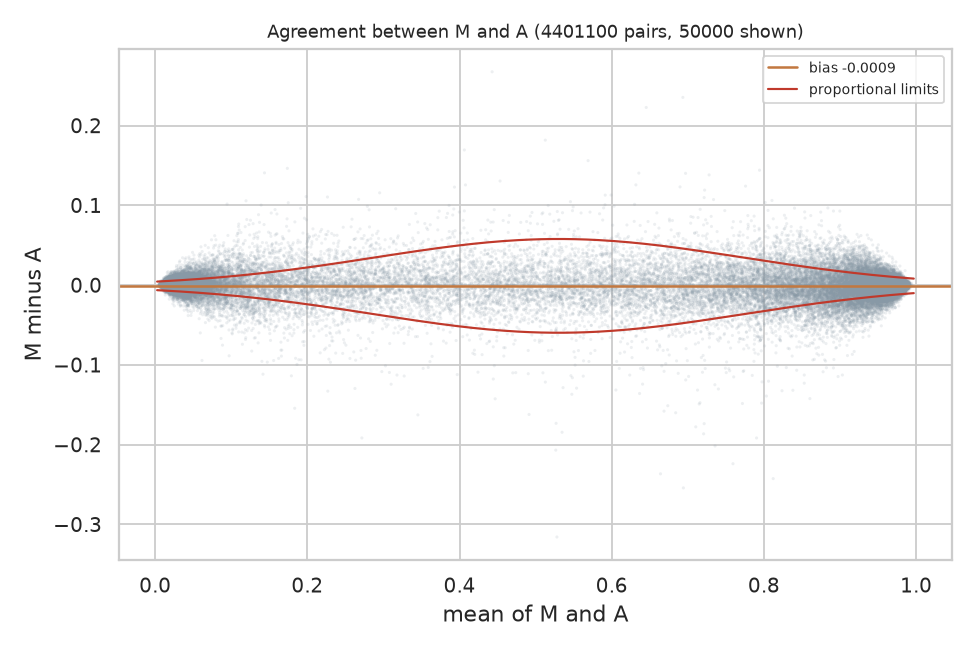
Bland Altman for MagNA Pure against Autopure, over all 4,401,100 paired values, with the variable limits the authors fitted. The bias line sits essentially on zero. The limits widen through the middle of the range and narrow at both ends, which is the behaviour of a bounded measurement and the reason flat limits do not describe it.
I put the canvas back to their method and kept that version. It is worth saying plainly: the first substantive result of reproducing this paper was confirming a methodological decision most readers would skim past.
---
What the study could not have seen
Here is the part I think matters, and it is arithmetic rather than opinion.
With ten donors and 440,110 simultaneous tests, the Benjamini Hochberg [5] threshold for the smallest p value in the set is 1.14e-07. The smallest p value actually present in their data is 7.6e-07. That is seven times larger than the threshold.
No site could have reached significance. Not because there was nothing there, but because the design could not resolve anything at that correction level.
Turned around into units anyone can picture: with this sample size, the median CpG would have needed a difference of about six percentage points of methylation to be detected. The differences that actually exist are around a quarter of one percentage point. A real effect twenty times larger than what is present would still have come back as "not significant".
This does not make their conclusion wrong. I think their conclusion is right. But "we found no significant differences" and "there are no meaningful differences" are different statements, and only the first one is supported by a test that could not have produced any other outcome.
To their credit, the authors say this. Their abstract contains the phrase "although this study is based on a small sample". My complaint is not that they hid it. It is that the hedge sits in one sentence of the abstract while the analysis is presented as though it could have found something, and most readers will take the analysis at face value.
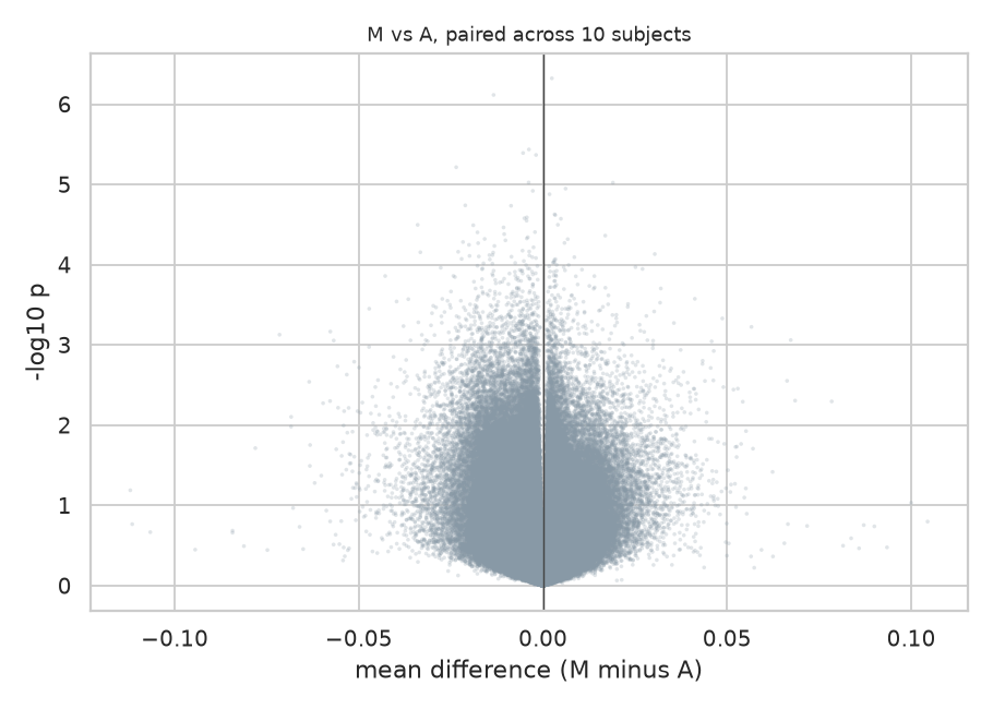
Effect size against evidence for all 440,110 sites. Nothing reaches the top of the plot, and the horizontal spread is narrow: the differences are small and none of them is well supported. A null result deserves a figure that shows this rather than an empty table, which reads as a broken analysis.
So I added a line to every one of those tests reporting the smallest difference it could have detected. It costs nothing to compute and it changes how a null result reads.
---
Asking the question they wanted to answer
If you want to claim two things are the same, a non significant difference test is the wrong tool. The two one-sided tests procedure [3] exists for exactly this. It tells you that you failed to distinguish them. Equivalence testing asks directly: are these two within a margin small enough not to matter?
The margin has to be set in advance and justified, because the whole procedure rests on it. I used 0.02 on the beta scale, two percentage points of methylation, on the grounds that this is the usual figure quoted for the technical noise of this array. A difference smaller than the measurement error is not a difference anyone can act on.
Across all 440,110 probes:
| Comparison | Equivalent within 0.02 | Median difference |
|---|---|---|
| MagNA Pure against Autopure | 81.9 percent | 0.0025 |
| Autopure against organic | 76.6 percent | 0.0028 |
| MagNA Pure against organic | 73.4 percent | 0.0030 |
This is a positive claim where the paper had the absence of one. Roughly four fifths of the epigenome can be shown equivalent between the two automated methods, at a margin tied to the instrument's own precision.
Two things must be said alongside it. The margin is a judgement: at 0.01 the figure drops to about half. And roughly a fifth of sites are in neither camp, neither shown to differ nor shown to be equivalent, which with ten donors is simply the honest answer.
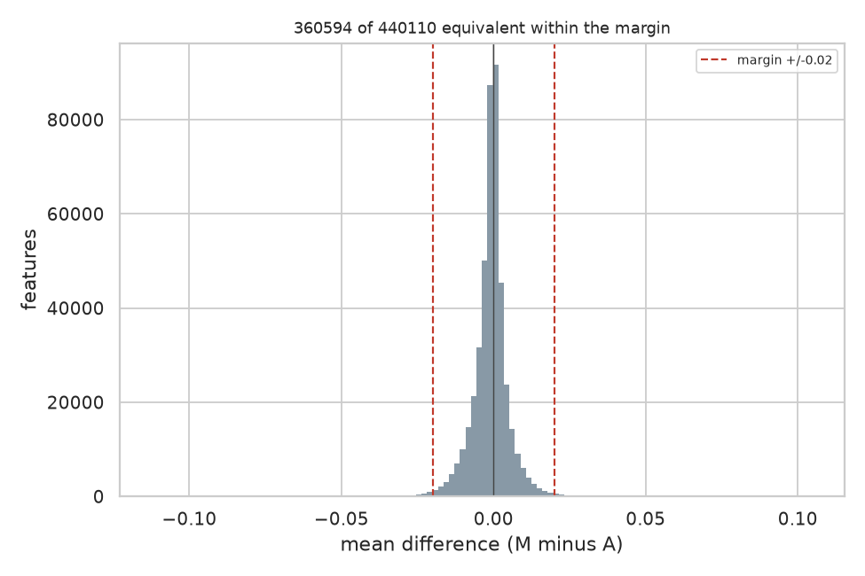
Every CpG's mean difference between the two automated methods, with the equivalence margin marked. Almost the whole distribution sits inside it, which is what 81.9 percent equivalent looks like. The tails are the sites this sample cannot decide about.
The ordering is worth noticing. The two automated methods agree most. Organic extraction agrees least with both. That is exactly what the authors described in words: "differences between organic extraction and each of the automated methods were in general larger than differences between the two automated extraction methods". Equivalence testing puts a number on an observation they could only state qualitatively.
---
Looking for something 440,110 separate tests cannot see
Testing every site independently is blind to a small shift shared by all of them. Each site pays the full multiple testing penalty while the evidence is spread across the whole array.
A global test does not have that problem. Compute one statistic over everything, then compare it against the same statistic computed on data where the labels have been shuffled in a way the design permits. For a paired design, the permutation is a sign flip within each donor: swap which method is called first. Ten donors give 1,024 distinct sign flips, and I drew 2,000 permutations.
| Comparison | p |
|---|---|
| MagNA Pure against Autopure | 0.094 |
| MagNA Pure against organic | 0.058 |
| Autopure against organic | 0.0155 |
Autopure against organic extraction shows a systematic difference across the array that no single site could demonstrate.
I ran this first on a subset with fewer permutations and got 0.033. At full scale and higher precision it came in at 0.0155. A signal that strengthens when you add data and precision is behaving like a real effect rather than noise.
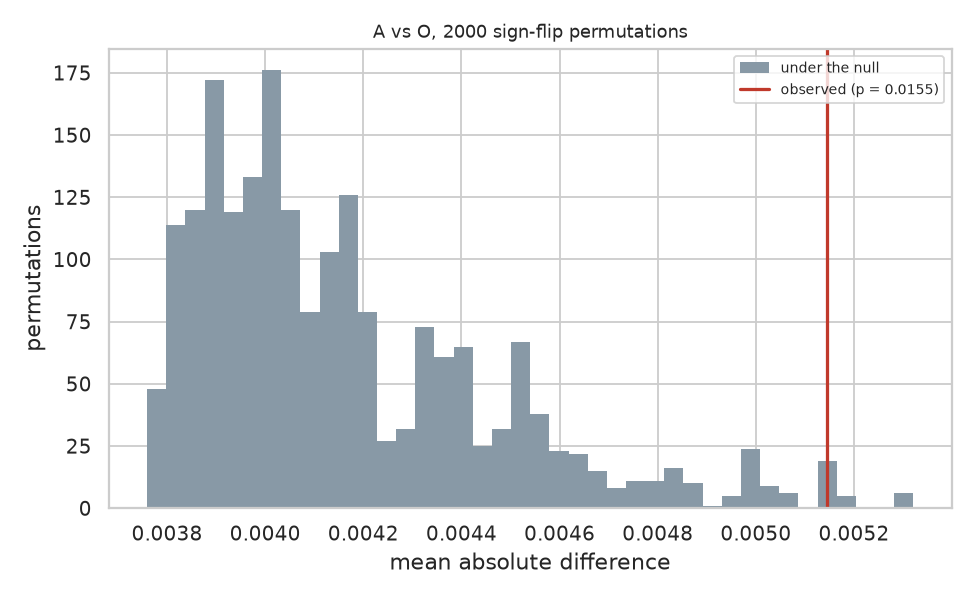
The statistic computed on 2,000 sign flipped versions of the same data, with the observed value marked. The observed statistic sits in the right tail rather than outside the distribution, which is what p equals 0.0155 looks like and why this is a signal rather than a demonstration.
The honest qualification: three comparisons were made and no correction was applied across them. Bonferroni corrected, 0.0155 times three is 0.047. It survives, but only just.
---
Regions rather than sites
Their fourth analysis looked for differentially methylated regions, runs of neighbouring sites moving together. A region level effect can exist where site level tests find nothing, because the evidence accumulates across positions.
I implemented the bump hunting approach of Jaffe and colleagues [4]: cluster probes that sit within 1000 bases of each other, find runs where the difference exceeds a cutoff, score each run by its area, then judge those scores against the largest run found in each of 2,000 permuted datasets. Judging against the largest run anywhere is what makes the error rate family wise, and it is the only correction that means anything when the regions were found by searching.
I should be clear that this is not the Bioconductor Bumphunter package. The clustering, the cutoff and the permutation null follow the same approach, but the smoothing is simpler, so the results will not be identical to theirs.
Across 153,239 clusters: zero significant regions for MagNA Pure against Autopure, zero for MagNA Pure against organic, and one for Autopure against organic.
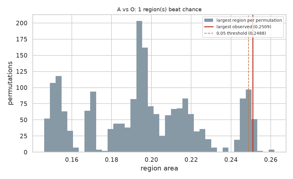
The largest region found in each of 2,000 permuted datasets, with the largest real region marked in red and the 5 percent threshold dashed beside it. The two lines almost touch. This figure is the honest picture of the finding: it clears the threshold, and it clears it by very little, with a stack of permutations sitting right at the boundary.
One region, area 0.25092 against a threshold of 0.24884: it clears by 0.8 percent. I reran it with eight times the permutations to see whether it was an artefact of a coarse null, and the threshold barely moved, from 0.24918 to 0.24884. The region clears it consistently.
I would not publish that on its own. As a fourth independent line pointing at the same comparison, it stops looking like chance.
---
The check that turns a null result into a finding
Their fourth analysis was a principal component analysis on the samples, tested against extraction method. I could not run it at first because my platform's PCA works across rows and this design needs the other orientation, one row per sample rather than one row per probe. So I built the transpose, and then the association test.
Principal components find the directions the samples actually vary along. The question worth asking is whether those directions line up with anything in the study design, because if the largest source of variation is the protocol then it is sitting inside every result the study reports.
Thirty samples, the fifty thousand most variable probes, ten components, each tested against extraction method and against donor, Bonferroni corrected across every test performed:
| Factor | Components associated, of ten |
|---|---|
| Extraction method | 0 |
| Donor | 9 |
This is the result I would put first if I were writing their paper again.
Nothing about the extraction protocol shows up in how the samples vary. But the person the blood came from shows up in nine components out of ten. The analysis is demonstrably capable of finding structure, because it finds the individual, and it does not find the protocol anywhere.
That is a different claim from "no significant differences". A null result alone leaves open the possibility that the method could not see anything at all. A null result standing next to a strong positive control on the same data, from the same test, closes it. The variation between two people is large and easy to detect. The variation introduced by choosing a different extraction kit is not there to find.
Four analyses, one ranking
The strongest thing here is not any single test. It is that four different analyses put the three comparisons in the same order, and that order is the one the authors described:
| MagNA vs Autopure | Autopure vs organic | MagNA vs organic | |
|---|---|---|---|
| Equivalent share | 81.9 pc | 76.6 pc | 73.4 pc |
| Permutation p | 0.094 | 0.0155 | 0.058 |
| Significant regions | 0 | 1 | 0 |
The two automated methods resemble each other. Organic extraction is the outlier. No single result carries that conclusion. The convergence does.
---
A confound I expected to find and did not
Their methods note that the blood sat for 2 hours before MagNA Pure extraction, 24 hours before Autopure, and 5 hours before organic. Extraction method is therefore confounded with storage time, which looked to me like a serious weakness when I first read it.
If storage time drove the differences, the comparisons would order by the size of the storage gap. They order exactly inversely. The 22 hour gap produces the smallest difference, and the 3 hour gap produces the largest. Spearman correlation of minus one.
Storage time does not explain the pattern. I am reporting this because I went looking for a flaw, did not find one, and think saying so is part of doing the exercise honestly.
---
What I did not reproduce
Their epigenetic age and cell composition estimates, which need reference data I did not assemble.
Their PCA also tested the components against sample position on the chip, and against per sample DNA yield and quality. None of those are in the deposited data, so I tested against extraction method and donor only.
Everything else in their paper is covered.
---
The part I actually care about
Here is the part nobody does, nobody likes doing, and which is hard to do anyway. Logging every step, every detail and every hidden parameter was never a human skill. We do not forget out of carelessness. We forget because there is no moment during the work when writing it down feels more important than the work, and by the time it matters the moment has gone.
Every run in this exercise was recorded as it happened: the analysis as it stood at that moment, a fingerprint of it, the random seed, the data, the results, who ran it, and what had changed since the previous run. Ten entries in all. Six were exploratory. Four I committed to.
Two entries in that record are worth pointing at.
Entry 3 carries the same fingerprint as entry 1. After testing the authors' rejected assumption and putting the analysis back, the record shows the two configurations were identical, rather than me asserting it.
Entries 5, 7 and 10 read "unchanged from the previous run: the same canvas, run again". Committing to a result you have just tested, without quietly adjusting anything first, is visible in the record.
I could have written this article from memory and you would have had to take my word for the sequence. Instead the sequence is a document, attached to this post, generated from what was logged rather than from what I remember. Every number above appears in it.
That is what I think reproducibility infrastructure is for. Not archiving finished work, but recording the path while you are still on it, including the parts where you were wrong.
---
Where this leaves the paper
Their conclusion was right, and it is now positively supported rather than merely unrefuted. Two analyses they did not run do that: an equivalence test, which turns a careful hedge into a statement about roughly four fifths of the epigenome, and a component analysis with a control in it, which shows the data carries a strong signal for the individual and none at all for the protocol. There is also a consistent signal separating organic extraction from the automated methods that their site level analysis was not able to resolve, and that deserves a larger cohort.
None of that is a criticism of the authors. They ran a careful study, published their data, described their methods precisely enough for a stranger to rebuild them six years later, and stated their own limitation in the abstract. That is more than most papers manage, and it is the only reason this exercise was possible at all.
The gap I am pointing at is not theirs alone. Equivalence testing is standard practice in clinical trials and almost absent from omics. Detection limits are almost never reported next to negative results. Both are easy. Neither is routine.
If you work on this array or on extraction protocols, I would like to hear whether the organic extraction signal matches what you see. The data is public, the analysis is described above, and I am happy to share the pipeline.
---
The analysis, as it actually looks
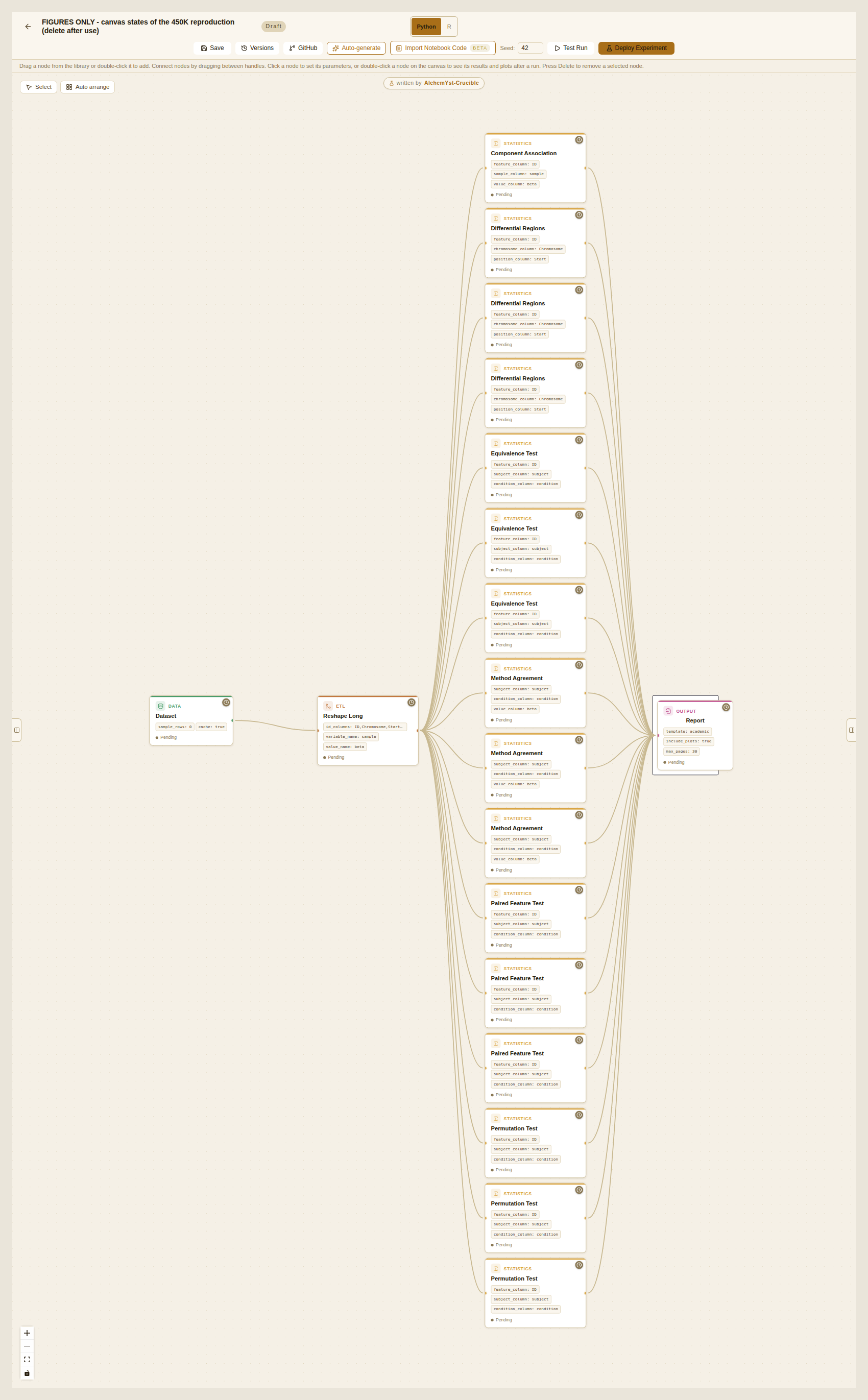
All four analyses on one canvas. The dataset on the left, the reshape that turns the column headers into a donor column and a method column, then sixteen statistical steps, then the report. Three of each test, one per pair of extraction methods, plus the component analysis. Every parameter that produced the numbers in this article is visible on the cards: the equivalence margin of 0.02, the 2,000 permutations, the 1,000 base clustering distance, the seed of 42 in the toolbar.
This is not a diagram drawn for the article. It is the thing that ran.
---
A note on the screenshots: the project discussion in this piece involves seven lab members. They are all my own accounts. I explain why, along with what could not be reproduced from this study and what I think that says about how research is published, in a follow up post.
References
[1] Hjorthaug HS, Gervin K, Mowinckel P, Munthe-Kaas MC. Exploring the influence from whole blood DNA extraction methods on Infinium 450K DNA methylation. PLoS ONE 2018;13(12):e0208699. doi:10.1371/journal.pone.0208699
[2] Bland JM, Altman DG. Statistical methods for assessing agreement between two methods of clinical measurement. The Lancet 1986;327(8476):307-310. doi:10.1016/S0140-6736(86)90837-8
[3] Schuirmann DJ. A comparison of the two one-sided tests procedure and the power approach for assessing the equivalence of average bioavailability. Journal of Pharmacokinetics and Biopharmaceutics 1987;15(6):657-680. doi:10.1007/BF01068419
[4] Jaffe AE, Murakami P, Lee H, Leek JT, Fallin MD, Feinberg AP, Irizarry RA. Bump hunting to identify differentially methylated regions in epigenetic epidemiology studies. International Journal of Epidemiology 2012;41(1):200-209. doi:10.1093/ije/dyr238
[5] Benjamini Y, Hochberg Y. Controlling the false discovery rate: a practical and powerful approach to multiple testing. Journal of the Royal Statistical Society Series B 1995;57(1):289-300. doi:10.1111/j.2517-6161.1995.tb02031.x
Methods applied upstream of the deposited data, by the original authors. Not rerun here: this reproduction begins from their preprocessed file, so these steps are taken on trust rather than checked.
Assenov Y, Muller F, Lutsik P, Walter J, Lengauer T, Bock C. Comprehensive analysis of DNA methylation data with RnBeads. Nature Methods 2014;11(11): 1138-1140. doi:10.1038/nmeth.3115
Teschendorff AE, Marabita F, Lechner M, Bartlett T, Tegner J, Gomez-Cabrero D, Beck S. A beta-mixture quantile normalization method for correcting probe design bias in Illumina Infinium 450k DNA methylation data. Bioinformatics 2013;29(2):189-196. doi:10.1093/bioinformatics/bts680
Data. Hjorthaug HS et al. Preprocessed Infinium 450K dataset. Zenodo, 2018. doi:10.5281/zenodo.1285774
A note on the implementations. The region search follows the approach in [4] rather than running the Bumphunter package: the clustering, the cutoff and the permutation based family wise correction are the same, the smoothing is simpler, and the outputs will therefore not match that package exactly. The equivalence test is the two one-sided tests procedure of [3] applied per feature, with the correction of [5] where stated. Everything else is standard and named where it is used.